Configuring acquisition

Welcome to this guide to the DataPlug, your HAI-P200-4G controller’s data acquisition feature. This tutorial shows you how to use our graphical configurator to collect, structure and publish data from your industrial equipment in a few clicks, over OPC-UA, Modbus TCP, Modbus RTU, S7-Com, BACnet/IP, NMEA 0183, or published by your own Node-RED flows. By the end of this guide, your data will be available on the internal MQTT broker, ready to be used by the Data-Explorer, by Node-RED or by your own applications.

Prerequisites

The HAI-P200-4G controller
HAI-OS

Configuration

Setting up the inputs

Modbus TCP

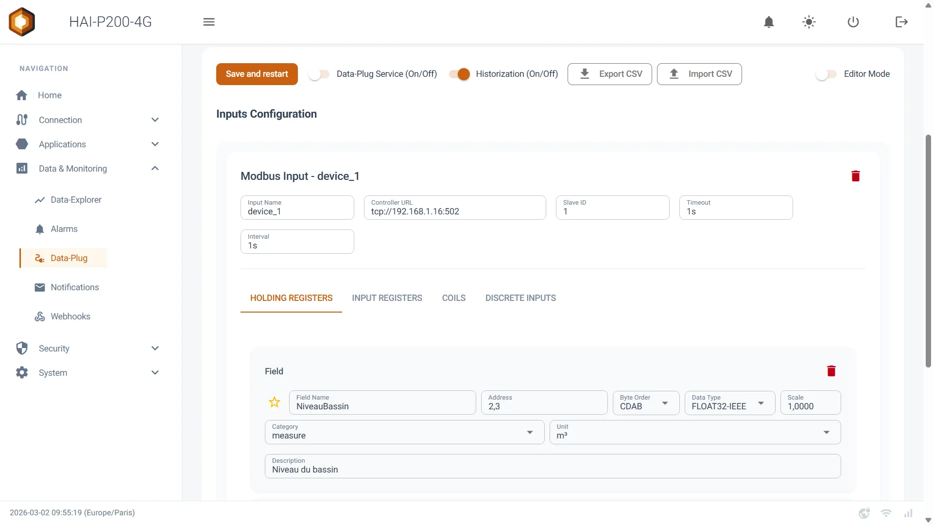
For Modbus, you can name the device using this protocol (Input Name), type in its URL together with its port (Controller URL), and select the slave identifier (Slave ID), its timeout and the data collection interval (Interval).

You can then add the fields whose value you want to retrieve. There are 4 kinds of field:

Holding Registers: code 0x03 (Read Holding Registers)
- Reading 16-bit words, read/write.
Input Registers: code 0x04 (Read Input Registers)
- Reading 16-bit words, read-only.
Coils: code 0x01 (Read Coils)
- Reading bits (booleans), read/write.
Discrete Inputs: code 0x02 (Read Discrete Inputs)
- Used to read bits (booleans), read-only.

To set up a Modbus field technically, so that it reads the right piece of information, you have to fill in the following:

Address: the numeric address of the register in the equipment’s Modbus table (0 or 100, for example). Note: if you choose a 32- or 64-bit data type, the interface automatically works out the addresses of the consecutive registers needed.
Data Type: says how to decode the value read (INT16 for a standard integer, FLOAT32-IEEE for a real, STRING for text, or BIT).
Byte Order: the Modbus standard does not define the word order for values larger than 16 bits, so it varies from one PLC manufacturer to another (AB, ABCD, CDAB). This setting puts the bytes back in the right order to obtain the correct value.
Scale: a multiplier applied automatically to the raw value read (type 0.1, for instance, to divide an integer value by 10 and simulate a decimal point).
Bit: this parameter only appears if you select the “BIT” data type. It isolates and reads a specific bit (0 to 15) inside a 16-bit register.

You can also name those fields and choose their contextualisation settings (category, unit, description). As for the fields’ unit: despite the large number of units offered, the one you want may not be there. You can then create your own unit by typing its name in the selection box and pressing the Enter key.

OPC-UA

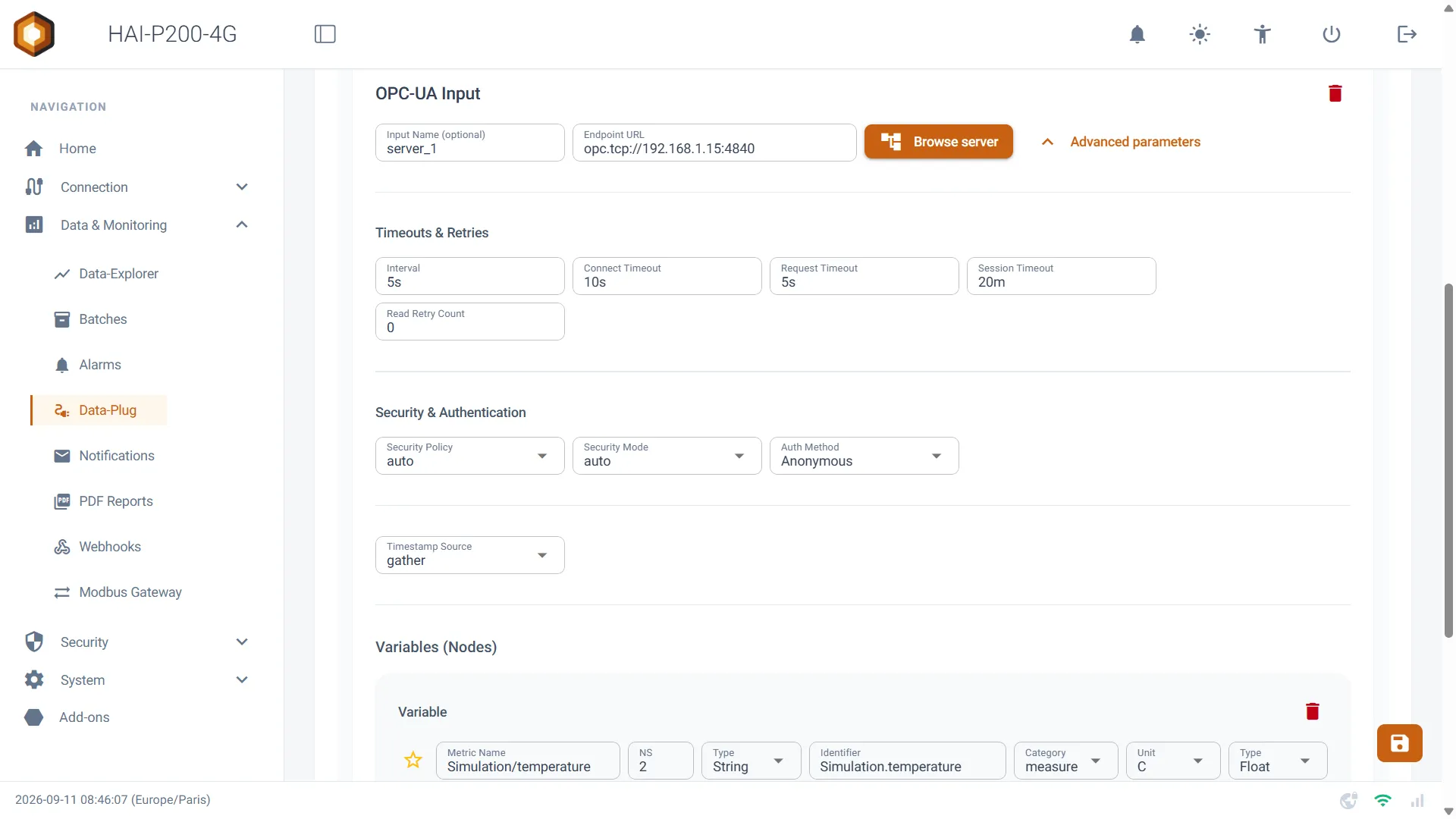
For OPC-UA, you can choose the input’s name (Input Name) as well as its URL with its port (Endpoint URL), in the opc.tcp://IP_ADDRESS:PORT_NUMBER format.

You can also configure the timeouts and retries. These are the fields you can change:

Interval (collection interval): this setting defines how often Telegraf queries the OPC-UA server to retrieve the data. It is the basic rhythm of the collection. If this field is set to ‘10s’, Telegraf asks for the values of every configured variable every 10 seconds.
Connect Timeout: this is the maximum time the client waits to establish the initial connection with the OPC-UA server. If the server does not answer the connection attempt within that delay (‘10s’, for instance), the connection is considered failed. It is the first door to get through.
Request Timeout: once connected, this delay applies to each individual request (reading or writing a variable). If the client asks for a sensor’s value and the server does not answer within that delay (‘5s’, for instance), the request fails, even if the overall connection is still active. This avoids waiting indefinitely for the answer to a single operation.
Session Timeout: this field defines the maximum time a communication session can stay idle. A session is a communication “context” between the client and the server. To stop the server from closing the connection for lack of activity, the client periodically sends “keep-alive” messages. This timeout guarantees that if the client and the server stop communicating for that long (‘20m’, for instance), the session is invalidated and will have to be re-established.
Read Retry Count: the number of times the client will retry reading a variable if the first attempt fails (because of a Request Timeout, for example). If this field is set to 3, on a read failure the client tries 3 more times before giving up and reporting an error. Setting it to 0 means there will be no retry at all.

You can also change the Security & Authentication section, which is crucial in OPC-UA, since it guarantees that your industrial data is protected against interception, alteration and unauthorised access. It is built on three pillars: the policy, the mode and the authentication method :

Security Policy: this setting defines which encryption algorithms will be used to secure the communication. It is the “how” of security.
- auto or None: no security. Data travels in clear. Only to be used for tests, or on a completely isolated network.
- Basic128Rsa15, Basic256, Basic256Sha256: these are predefined sets of increasingly robust algorithms. The stronger the policy, the more secure the communication (with a minimal impact on performance).
Choosing a policy other than None requires certificates (.pem) for the client and the server, in order to establish a secure connection.
Security Mode: this setting defines what is protected using the chosen security policy.
- None: nothing is secured.
- Sign: each message carries a digital signature. That guarantees integrity (the message has not been altered on the way) and authenticity (you are sure who sent it). The message’s content is not encrypted, however, and stays readable.
- SignAndEncrypt: this is the highest level. Messages are both signed AND encrypted. That guarantees integrity, authenticity and confidentiality (nobody can read the messages’ content).
Auth Method: this setting defines how a user or an application proves its identity to the server.
- Anonymous: no authentication is required. Any client can connect, although the security rules (encryption) may still apply.
- UserName: the client has to provide a valid user name and password to be allowed to connect.
- Certificate: authentication is done through the client’s digital certificate. It is a very secure method.

You can also select the source of the timestamp the Data-Plug will transmit.

Then you can add your various variables (called “nodes” in OPC-UA). Unlike Modbus or S7, which use classic memory addresses, OPC-UA uses a specific addressing scheme that you have to fill in:

Namespace (index): the numeric index of the namespace (2 or 3, for example) defined in the OPC-UA server to organise and separate the variables.
Identifier Type: says what format your variable’s identifier is in. It can be numeric (i), a string (s), a GUID (g) or an opaque format (b).
Identifier: the exact identifier (the name or the number) of the variable in that namespace (1002 for a numeric type, or path.to.my.variable for a string type).

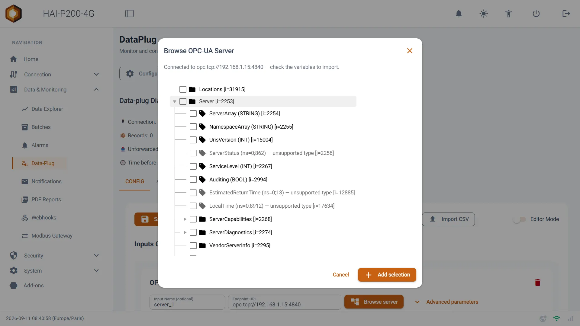
Browsing the server from the interface (Browse server)

Rather than typing the Namespace / Identifier Type / Identifier triplet in by hand, click Browse server, next to the endpoint URL. The configurator connects to the server with the parameters already entered (endpoint, security, authentication, certificates) and displays its tree, pre-loaded 6 levels deep.

Tick the variables you want — only Variables with a usable type (BOOL, INT, FLOAT, STRING) can be ticked — then confirm. Each imported variable arrives with its full BrowseName path as its name (Plant/Line1/Temperature, for example), along with its description and its type as read from the server.

The Browse OPC-UA Server window: the tree of server opc.tcp://192.168.1.15, a checkbox in front of each node, variables with an unsupported type greyed out, Cancel and Add selection buttons

Certificates

As soon as the security policy is no longer None, the Generate client key pair button creates and downloads a self-signed client certificate (10-year validity) straight from the interface: there is no need to build one separately. The Trusted Server Certificate field additionally lets you pin the server’s certificate, so that only that one is accepted.

Tip: finding your OPC-UA parameters easily with UaExpert

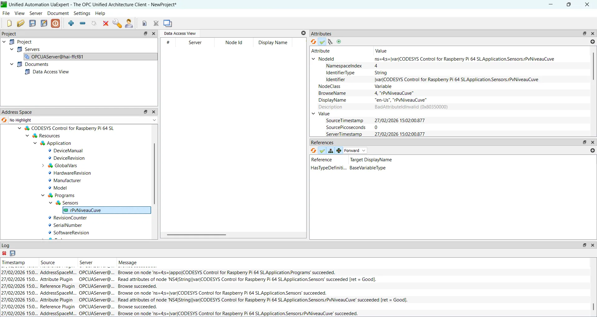
Using that tool, we can see that the fields have to be written this way in the Data-Plug:

Namespace: 4
Identifier Type: s (String)
Identifier: |var|CODESYS Control for Raspberry Pi 64 SL.Application.Sensors.rPvNiveauCuve

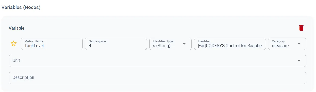
You can also set each variable’s display name, category, unit and description.

S7

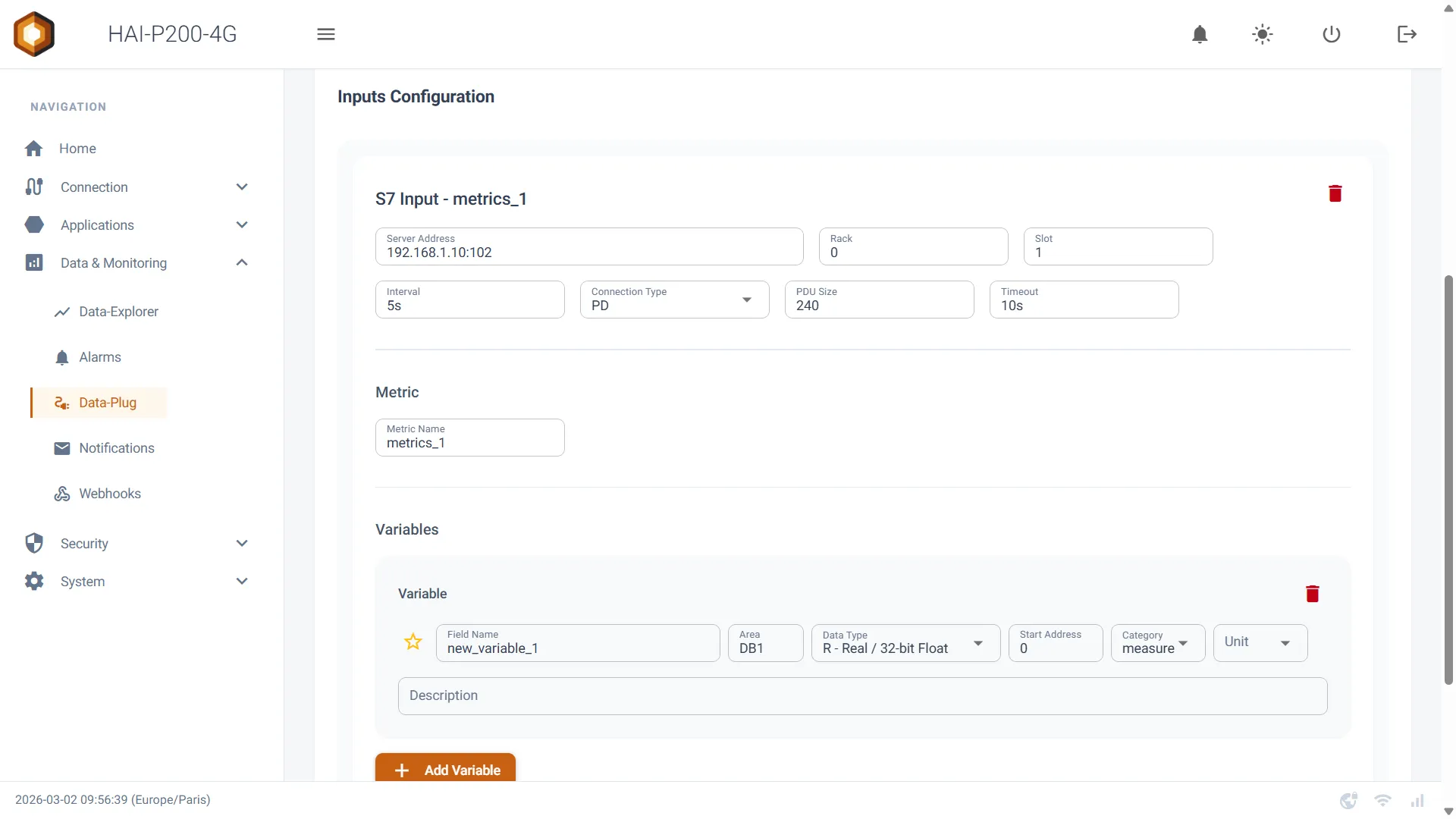
For the S7 protocol, you can enter the server’s IP address and its port (Server Address), along with its rack and its slot. You can also enter the type of communication (Connection Type) to establish with the PLC. The options are:

PD: for connections to “Processing Devices” (CPUs). This is the most common type.
OP: for connections to “Operator Panels” (HMIs).
basic: for basic connections with simpler communication modules.

You can then enter the pdu_size, which is the maximum size (in bytes) of the data packets (PDU — Protocol Data Unit) exchanged with the PLC. A larger size can improve performance but has to be supported by the PLC. The default value is 240.

You can then configure the Timeout, as well as the Interval, which defines how often Telegraf should query the PLC. That delay between collections is expressed with a time unit (5s, for example).

Finally, you can choose the metric’s name and add your variables below it.

When you add a variable, you can set its name (Field Name), its category, its unit and its description. You also have to give its address, using the following parameters:

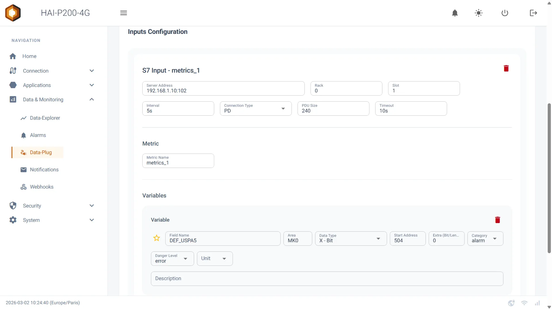
Area: the memory area the variable is in (DB1 for data block 1, MK0 for variables addressed as %M).
Data Type: the variable’s data type (R for Real/float, I for Integer, X for Bit, S for String).
Start Address: the starting address of the word or the byte in the memory area.
Extra (Bit/Length): an additional parameter that depends on the data type:
- For type X (Bit), it is the bit number (0 to 7).
- For type S (String), it is the length of the string to read.
- For the other types, this field is not used.

The case of a variable addressed as %M:

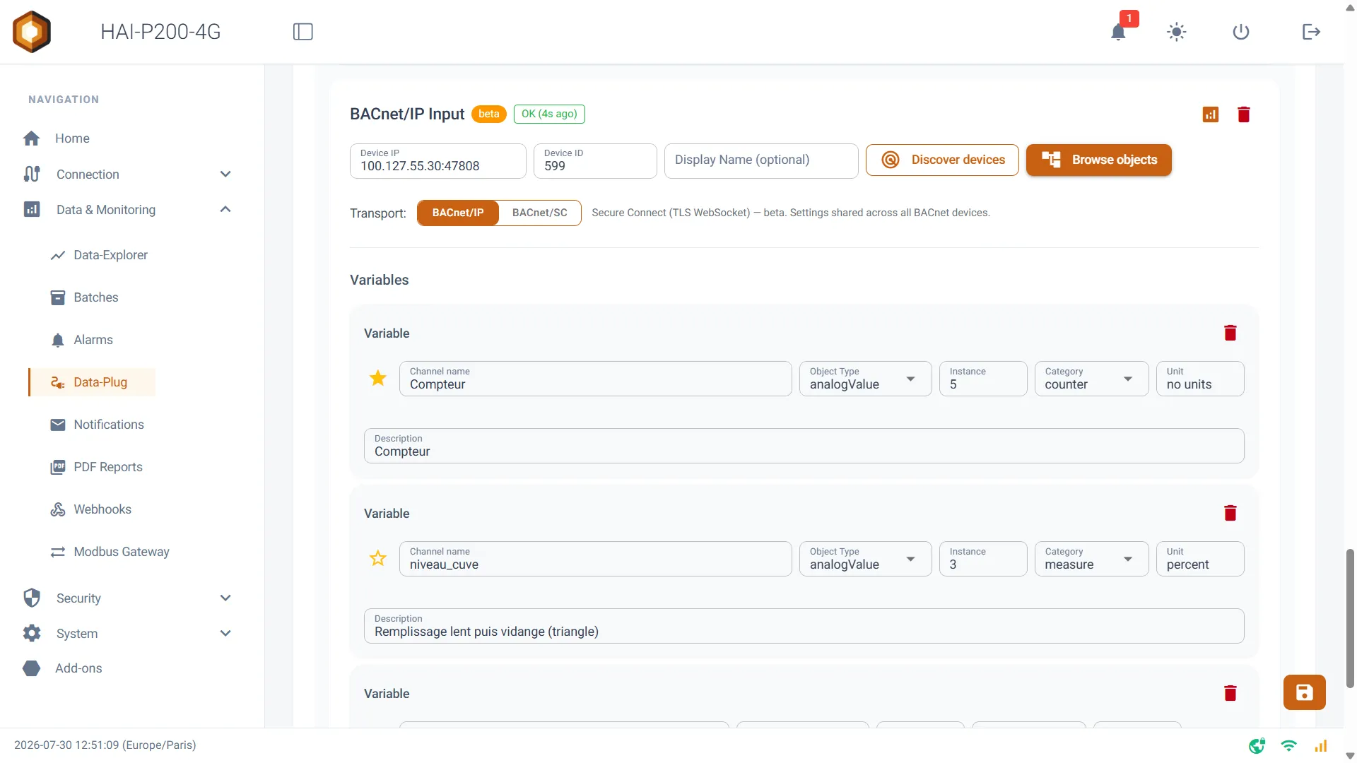
BACnet

The BACnet/IP protocol collects data from your building management equipment (HVAC, lighting, metering).

Declaring a device

Each BACnet card corresponds to one device:

Device IP: the device’s IP address.
Device ID: the BACnet device identifier (Device Object Identifier).
Display Name (optional): a readable name to find your way around.

A status badge at the top of the card continuously shows the collector’s situation: Stopped, Disconnected, OK with the age of the last reading, or the number of errors encountered.

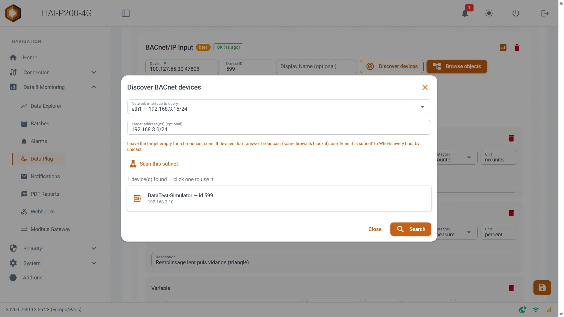
Finding your devices automatically (Discover devices)

Rather than typing the address and the identifier in by hand, click Discover devices. A window opens to start a search on the network:

Network interface to query: choose the network interface to search on. The interface matching the address already entered is preselected.
Target address(es) (optional): leave this field empty for a broadcast search, which is the simplest method. If your devices do not answer (some firewalls block broadcasts), enter an address, a CIDR range or a comma-separated list to query them one by one.
Scan this subnet: automatically fills the target field with the chosen interface’s subnet, to query each host individually.
Fill Tailscale peers: on a VPN interface (point to point), broadcasting does not work. This button fills in the list of connected Tailscale peers, to be queried directly.

Click Search: the devices found are shown as a list. Click one of them and its address, its identifier and its name are copied into the card.

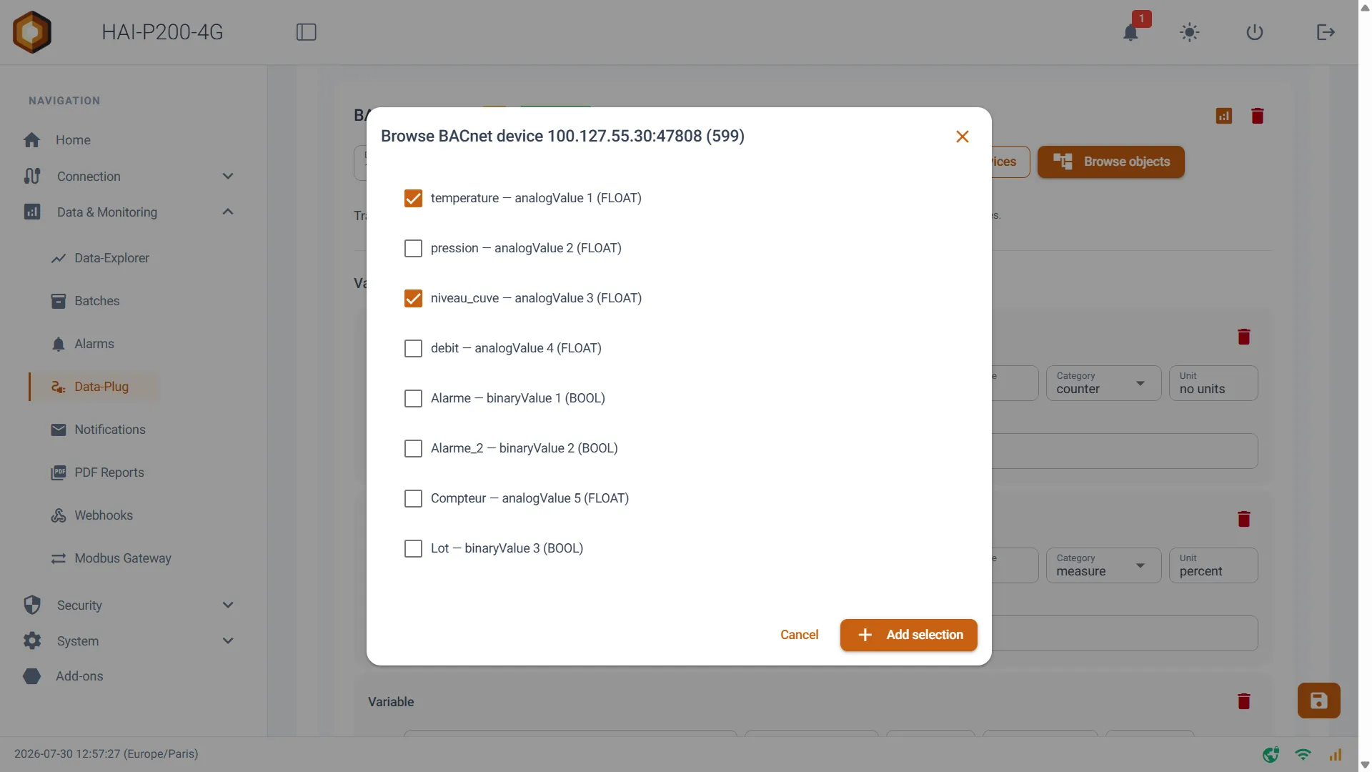
Adding variables (Browse objects)

The Browse objects button queries the device and lists its objects. Tick the ones you are interested in, then click Add selection: the variables are created with their object type, their instance, their value type, and — when the device provides them — their unit and their description. The category is initialised to measure: adjust it if necessary.

You can also click Add Variable to enter a variable by hand:

Channel name: the variable’s name in HAI-OS.
Object Type: the BACnet object type, among analogInput, analogOutput, analogValue, binaryInput, binaryOutput, binaryValue, multiStateInput, multiStateOutput, multiStateValue.
Instance: the object’s instance number.
Unit: note that on BACnet this field is free text, with no dropdown and no unit creation as on the other protocols.

The value type is deduced automatically from the object type: analog objects give a decimal number, binary ones a boolean, multiState ones an integer.

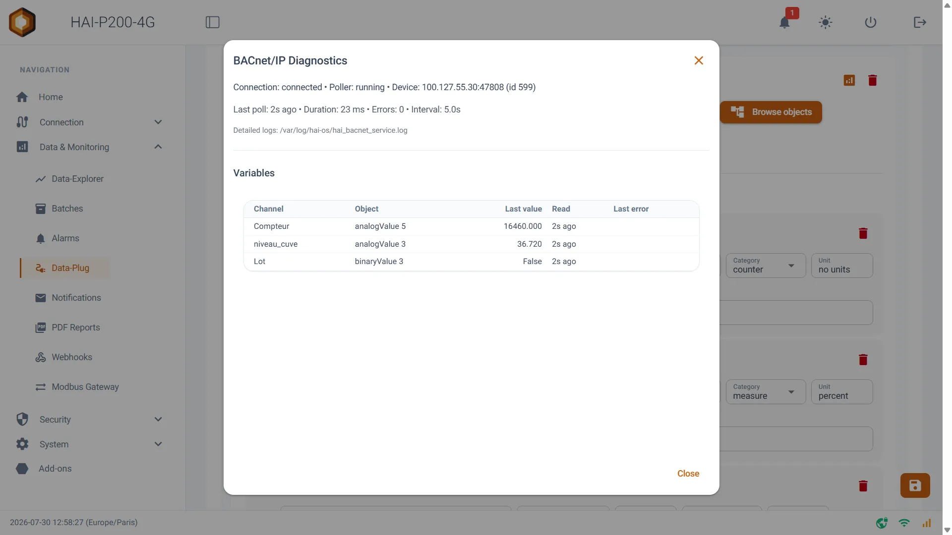
Per-device diagnostics

The chart icon at the top of the card opens the BACnet/IP Diagnostics window, updated every 2 seconds: connection state, collector state, date and duration of the last poll, number of errors, polling interval, and a row-by-row table giving each variable’s last value, its age and its last error. The detailed logs are in /var/log/hai-os/hai_bacnet_service.log.

BACnet/SC (beta)

A Transport selector offers to switch from BACnet/IP to BACnet/SC (Secure Connect), which routes the exchanges through a TLS tunnel to a hub. This setting is global to all your BACnet devices and only appears on the first card. In Secure Connect mode, devices are reached by their Device ID through the hub: the Device IP field disappears and the discovery and browsing functions are not available. The tunnel’s parameters (hub URL, client certificate and key, hub certificate) are entered in the same section.

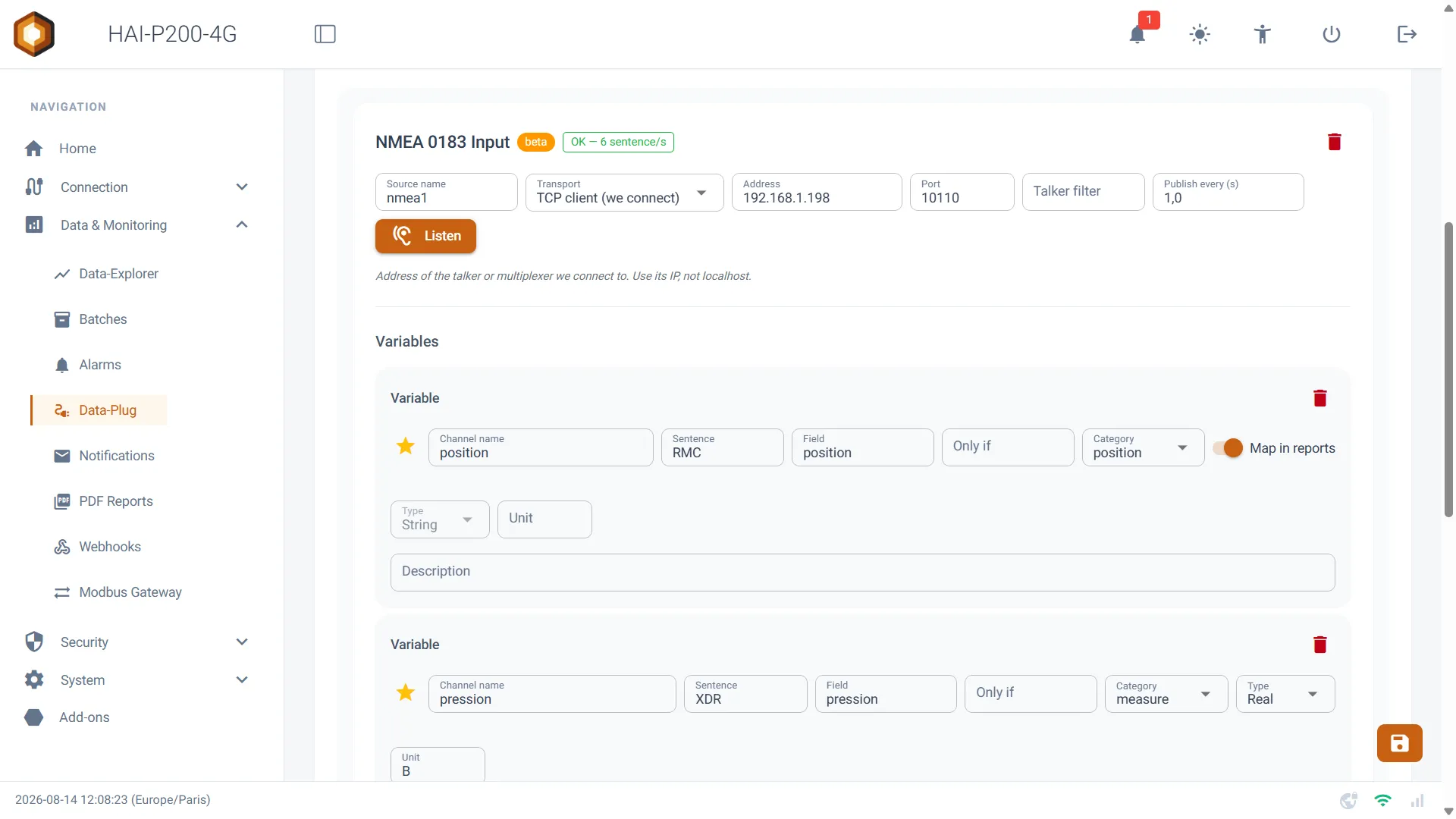
NMEA 0183

The NMEA 0183 protocol collects the sentences emitted by marine navigation and measurement equipment (GPS, echo sounder, wind vane and anemometer, navigation computer).

Declaring a source

Each card corresponds to a talker or to a multiplexer:

Source name: a readable name to find your way around.
Transport: TCP client (we connect) — the controller connects to the equipment; TCP server (they connect) — the equipment connects to the controller; UDP (listen) — the controller listens for datagrams.
Address / Bind address: as a TCP client, the equipment’s address (its IP, not localhost). As a TCP server or in UDP, the listening address — leave it empty to accept on every interface. The label and the help text below the field adapt to the chosen transport.
Port: the link’s port.
Talker filter: optional, to keep only one emitter (GP or II, for example).
Publish every (s): a talker emits 1 to 10 sentences per second. Only the last value of each variable is published, at this rate.

A status badge at the top of the card continuously shows the situation: Stopped, Disconnected with the reason, or OK with the reception rate in sentences per second. A source that is connected but silent shows up as a rate of zero.

Serial equipment: NMEA 0183 is originally a serial protocol. An RS232/RS422 talker connects through an external serial-to-Ethernet converter, configured to present the stream over TCP or UDP.

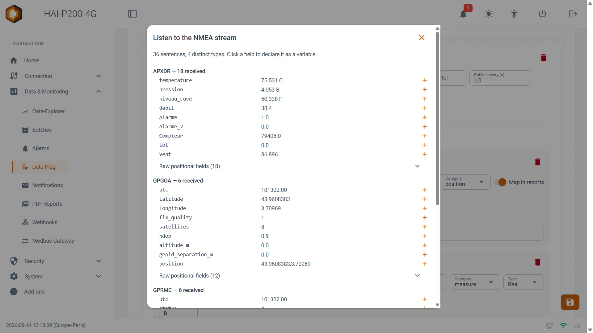
Adding variables with listen mode (Listen)

The Listen button listens to the source for a few seconds and shows the sentences received, decoded field by field. Each recognised field can be added as a variable in one click, with its unit when the sentence carries one. Fields the decoder cannot name stay available under “Raw positional fields”, read by their position in the sentence — beware, that position can vary from one manufacturer to another.

You can also click Add Variable and enter:

Channel name: the variable’s name in HAI-OS.
Sentence: the sentence type. Three letters match any emitter (RMC), five letters pin a single one down (GPRMC).
Field: the field to extract from the sentence.
Then the usual parameters: value type, category, unit, description.

Position on a map

From the latitude and the longitude of one and the same fix sentence (RMC, GGA, GLL), the decoder builds a composite position field. A variable declared on that field automatically takes the position category and the STRING type: the Data-Explorer then shows it as a track on a map rather than as a curve, over the selected period and live.

If that variable is marked as a favourite, a Map in reports switch appears: it adds the track to the PDF and e-mail reports. The map background is downloaded at generation time; with no Internet, the track is still drawn, on a neutral background.

Internal MQTT (Node-RED)

This input does not go and fetch the data: it receives it. It lets you declare variables in the Data-Plug whose values are published by an external MQTT client — a Node-RED flow, a home-made script, a third-party SCADA. Your data then benefits from everything else the Data-Plug offers: historisation, categories, favourites, alarms, reports and the Data-Explorer.

This is the way to go for any equipment whose protocol is not natively supported: you do the collection in Node-RED, and the Data-Plug takes over.

Only one input of this kind can exist on the controller. Declare as many variables in it as you need, filling in each one’s Channel name, value type, category, unit and description.

Publication format

A help button on the card recalls the expected format. Publish to the local broker localhost:1883 (with no authentication), on a topic starting with data/all/:

{
  "name": "<channel_name>",
  "fields": {
    "value": <value>
  },
  "timestamp": <epoch_ms>
}

name: must match the Channel name declared on the card exactly. It is this field, not the topic, that identifies the variable.
fields.value: a number, a boolean or a string.
timestamp: a Unix timestamp in milliseconds.

Any topic matching data/all/# is accepted. Telegraf plays no part in this chain.

Modbus RTU

To set up a connection using the Modbus RTU protocol, you first have to go to the configuration page dedicated to that protocol in your controller’s interface. That page lets you define your equipment’s serial communication parameters (serial port, transmission speed or baud rate, parity, data bits and so on).

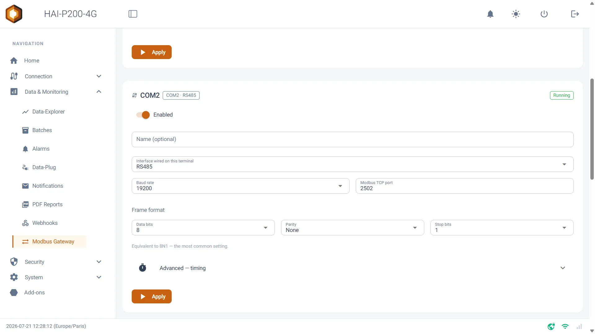
Once the serial link is established on that dedicated page, adding your device and collecting its data works exactly as for Modbus TCP. You just add it in the graphical configurator as an ordinary Modbus input.

To configure your variables, go back to the detailed explanation in the Modbus TCP section. You apply exactly the same method there to:

Select the field type: Holding Registers, Input Registers, Coils or Discrete Inputs.
Fill in the technical parameters: Address, Data Type, Byte Order, Scale or Bit.
Apply the business context: the variable’s name, category (Measure, State, Alarm, Counter), unit and description.

Putting the data in context

The anatomy of a variable When you add a variable in the Data-Plug, you have to configure two broad kinds of parameter:

The addressing (technical) parameters: they are specific to the chosen protocol and are what read the raw data in the equipment (the Address in Modbus, or the Namespace in OPC-UA).
The contextualisation (business) parameters: they are common to every protocol. They are what give the raw data meaning, and tell the system how to process and display it.

General information (the variable’s identity) For every variable added, whatever its protocol, you have to give its identity:

Name: the unique name that will be used to identify the data across the whole system (Motor_Temp, Tank_Level). Be clear and precise, because it is that name which appears in your charts and your alarms.
Unit: the measurement’s physical unit (°C, bar, m/s). Tip: although a very long list of units is offered in the dropdown, you can create your own by typing its name and pressing the Enter key.
Description: a free text field, very useful for documenting the variable’s context (“Temperature probe on the north discharge pipe”, for instance). This description is visible in the alarm notification e-mails and in the reports, to help with diagnosis.

When you create a variable (whether in Modbus, OPC-UA, S7, BACnet, NMEA 0183 or Internal MQTT), you have to assign it a Category. That choice is essential, because it tells the system how to process, aggregate and display the data in the charts and the reports:

Measure: for analogue values that vary continuously (temperature, pressure, level, speed). In the Data-Explorer, this category of variable is automatically shown as a curve.
State: for discrete or boolean values (a machine running or stopped, a valve open or closed). The data is shown as a step chart, to make state changes clearly visible in the Data-Explorer. Only value changes are published (deduplication).
Alarm: similar to the “State” category (a binary value, 0 or 1), but this category additionally triggers the alarm monitoring and notification system.
Counter: for variables that only ever increase over time (kWh energy meters, totalised water volume, part counters). The Data-Explorer shows these variables as consumption histograms over a given period.
Position (NMEA 0183 protocol only): for variables carrying a GPS point, that is, a latitude/longitude pair from one and the same navigation sentence. Its value is always a string, and the Data-Explorer shows it as a track on a map rather than as a curve. This category is only offered on NMEA 0183 variables.

To mark a variable as a favourite, click the star on the left. Favourite variables are transmitted both on the data/all topic and on the data/favorites topic. Favourite variables can also be found in the hai_vars table of your SQLite database.

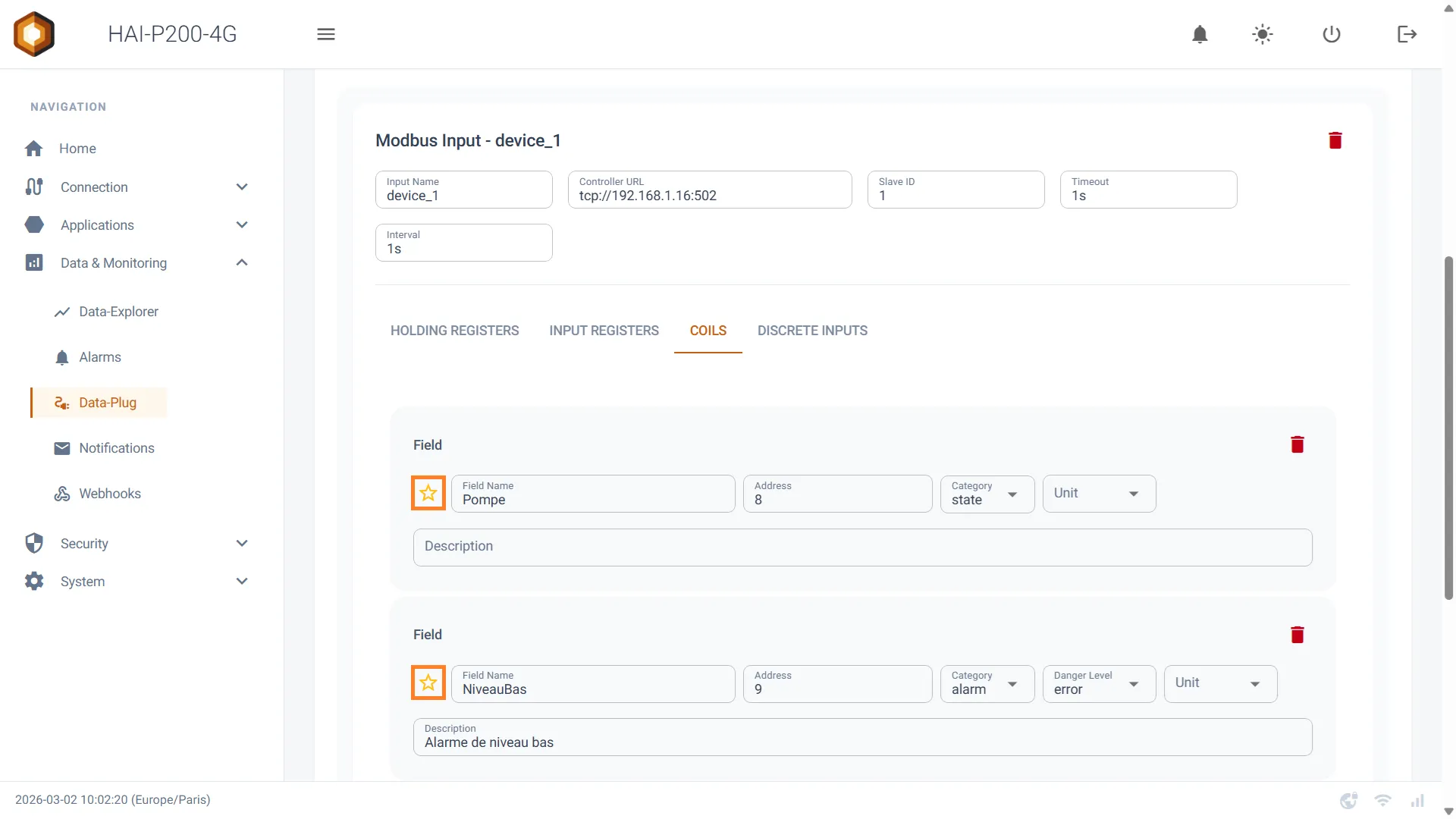
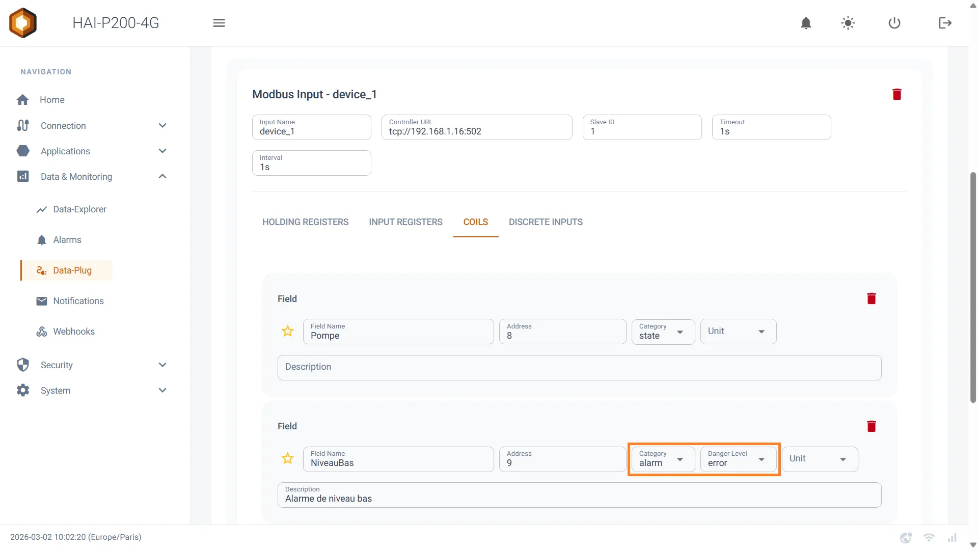
When you declare a variable as an alarm, an extra field appears, letting you choose the alarm’s type. By default it is an info, but you can also set it to warning or error. You can also create your own categories by typing their name and pressing the Enter key.

Additional settings

Depending on the category chosen, three extra settings can appear on the variable’s row.

Compute RCA (Alarm category variables)

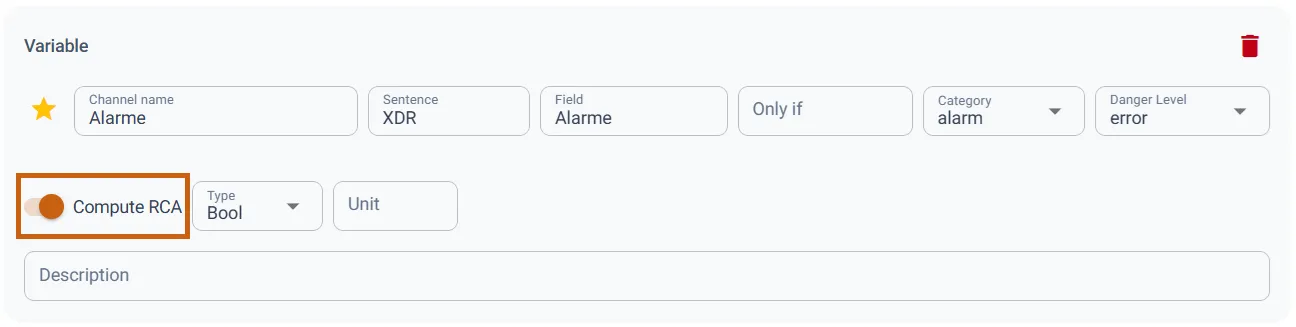
This switch, on by default, determines whether root cause analysis (RCA) is computed for that alarm. When it is off:

the RCA analysis button no longer appears next to that alarm on the Alarms page;
the notification e-mail sent for that alarm no longer contains the ranking of the most impacted variables, nor the associated charts.

The alarm is of course still detected, historised and notified: only the analysis is set aside. This is the setting to use for alarms whose automatic diagnosis you already know brings nothing, or to lighten the notifications of a frequent alarm.

Batch (batch identifier)

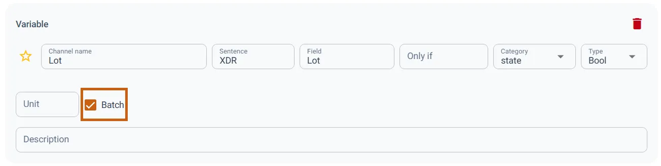
This box designates the variable that carries the batch identifier (a manufacturing number, a works order number, or simply a “production running” boolean). It is from its value changes that the Batches page rebuilds your batches:

a boolean variable: a batch is each period during which the value is 1. Periods at 0 are not batches;
an integer or text variable: each distinct value makes up a batch, which ends at the next value change.

The box is only offered on boolean, integer or text variables — a decimal value cannot serve as an identifier. Only one variable at a time can play that role: as soon as you tick one, the box disappears from all the others. Untick it to make the choice available again. This setting takes effect immediately, without waiting for Save and restart.

Map in reports (Position category variables marked as favourites)

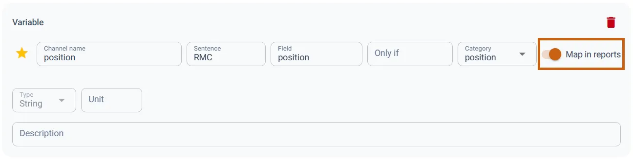
Adds the variable’s GPS track to the PDF and e-mail reports. The switch only appears if the variable is both in the Position category and marked as a favourite (⭐), since the reports only cover favourites. The map background is downloaded when the report is generated: with no Internet access, the track is still drawn, on a neutral background.

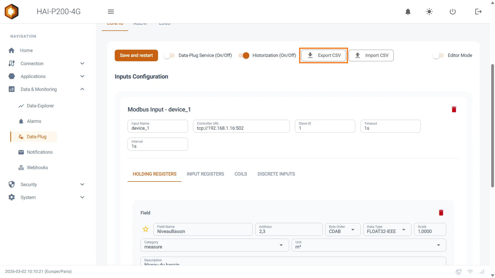
CSV import / export

To save you time when configuring many variables (Modbus, OPC-UA, S7, BACnet, NMEA 0183 or Internal MQTT), the configurator includes a CSV import/export feature. Rather than typing your dozens of variables into the form by hand:

Configure one or two variables as an example through the interface.
Click the Export CSV button (at the top of the Config tab).
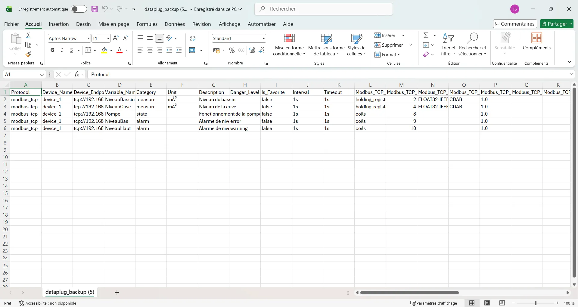
Open the downloaded file in Excel or a spreadsheet, copy and paste your rows and edit your variables quickly.
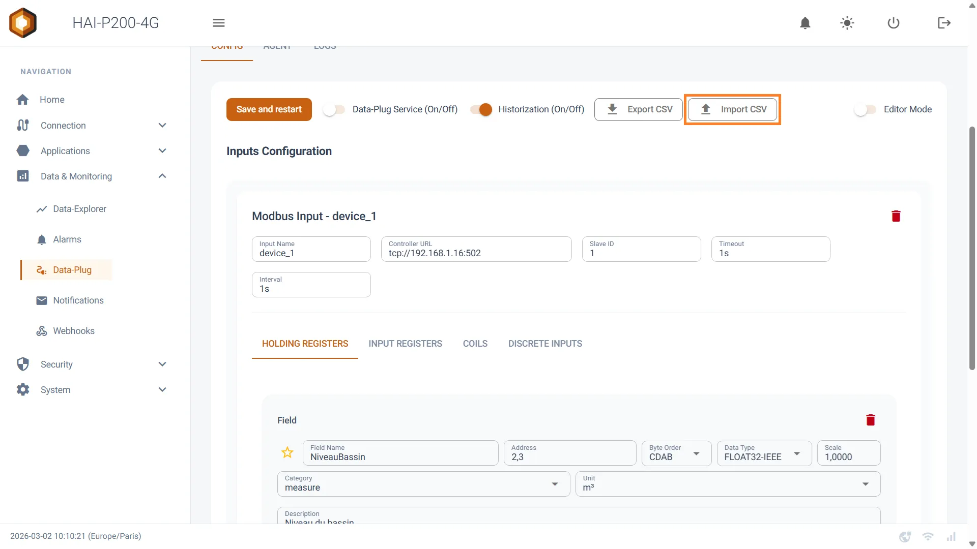
Click Import CSV to load your whole configuration in a flash.

Exporting historised data (Data Export tab)

The Data Export tab lets you download the data recorded over a period of your choosing:

From / To: the start and end dates and times. The last 7 days by default.
Favorites only: limits the export to your favourite variables (⭐).
Export CSV: generates and downloads the file.

If no data exists over the requested period, a message tells you so and no file is downloaded.

Setting up the agent

Open the Data-Plug page. The agent’s settings page is shown directly:

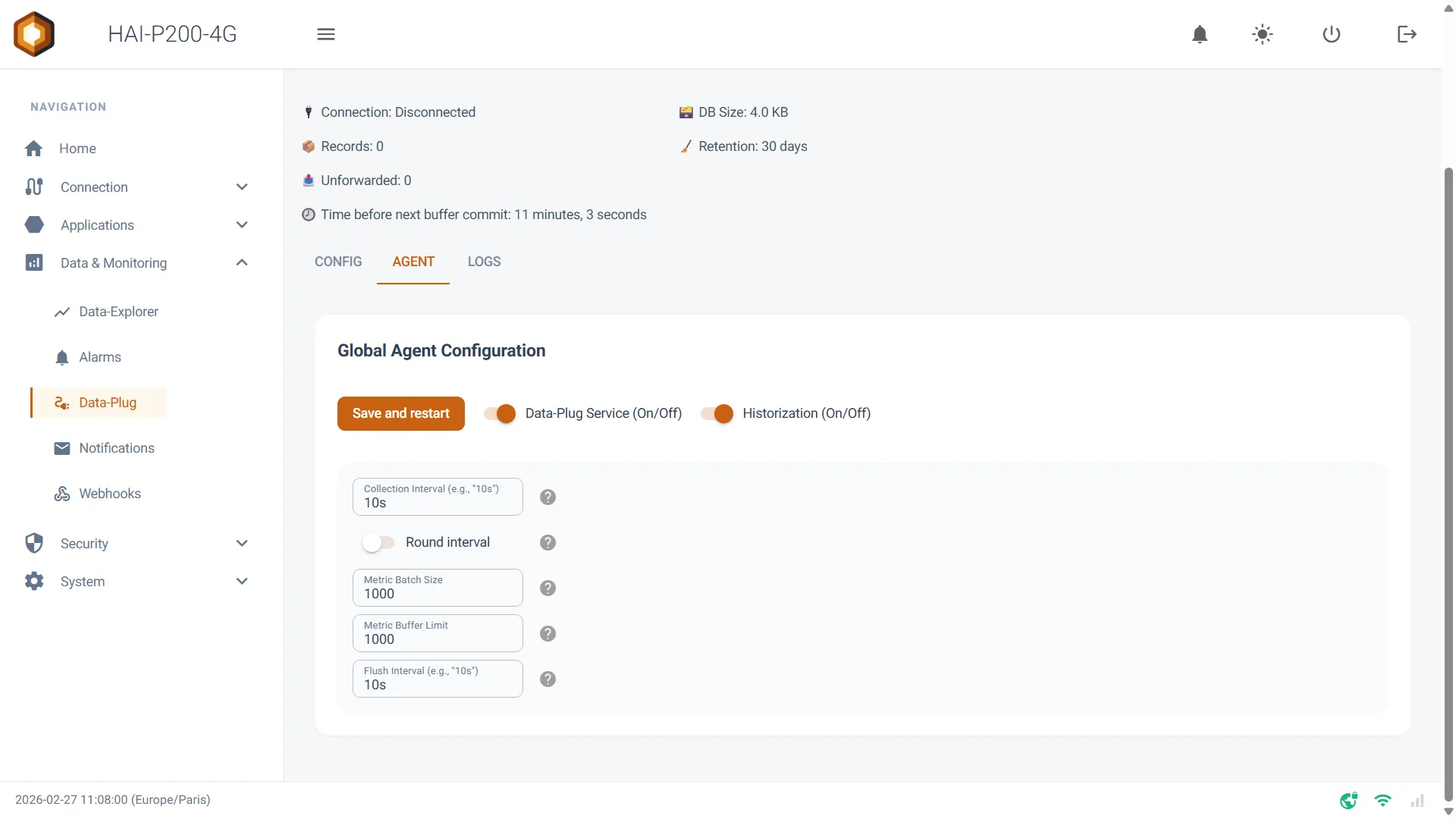
Here are the 5 key parameters that drive the agent’s behaviour:

Collection Interval: Telegraf’s collection rhythm. It defines how often (every 10 seconds, for example) the agent queries the data sources. A short interval gives more precision but increases the load.
Round Interval: once enabled, it synchronises the timestamps on round intervals (10:00:10, 10:00:20). The aim is to tidy the data up and make charts easier to align, especially when comparing several servers.
Metric Batch Size: the size of the data “parcel”. Telegraf groups metrics until it reaches this size, then sends everything in one block. Increasing this value optimises the network by reducing the number of transmissions.
Metric Buffer Limit: the safety buffer. If the destination is unreachable, Telegraf stores the metrics here so as not to lose them. This limit protects the agent from excessive RAM usage. If the buffer is full, the oldest metrics are dropped.
Flush Interval: a maximum sending delay. It forces the data out after a certain time, even if the “parcel” (Metric Batch Size) is not full. That guarantees that data, however sparse, does not stay stuck in the agent for too long.

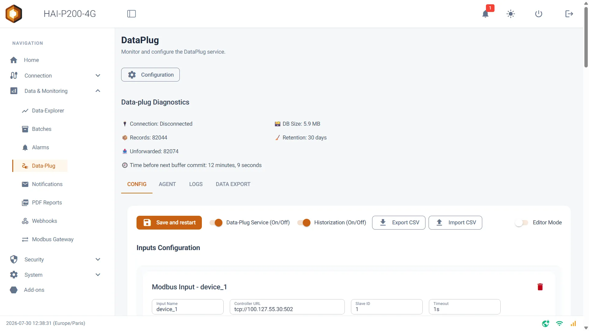
Diagnostics

At the top of the Data-Plug page, the Data-plug Diagnostics banner permanently shows the health of the collection. It is the first place to look when data seems to be missing. It refreshes automatically every 15 seconds.

🔌 Connection: the state of the Data-Plug’s connection to the broker (Connected / Disconnected).
📦 Records: the total number of records in the local database.
📤 Unforwarded: the number of records not yet transmitted to the cloud gateway. A rising value means the remote destination is unreachable — the data is not lost, it is waiting.
🕗 Time before next buffer commit: the time left before the buffer is next written to the database. This line disappears when historisation is disabled.
🗃️ DB Size: the size of the database file.
🧹 Retention: the configured data retention period, in days.

Saving and restarting

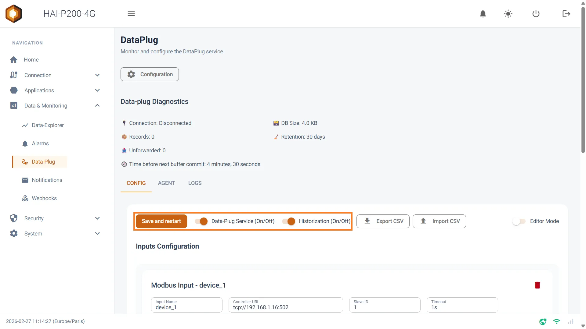
To save, click Save And Restart. This automatically restarts the Data-Plug. You can also switch it on and off by clicking Data-Plug Service (On/Off), or switch historisation on and off by clicking Historization (On/Off) (more details are available in 🔝 Store & Forward configuration).

Remember to save when you change page or view (between the form and the editor mode, for example).

Logs

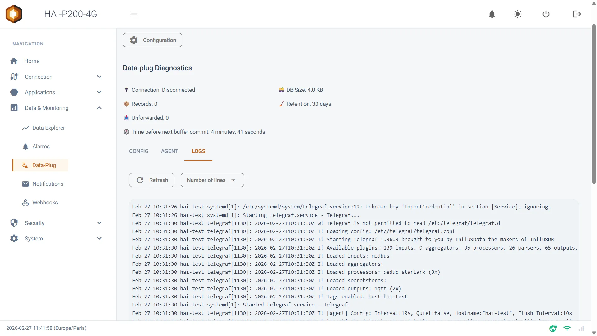
A tab on the Data-Plug page lets you view Telegraf’s logs. You can choose the number of lines to display and refresh the page easily.